Some Higher Dimensional Fractals

Fractals are geometric sets with self-similar structure. The interesting part is that this behavior usually comes from very compact iteration rules, so a small formula generates very high visual complexity. ^{1 2}

Sierpinski Triangle

The 2D Sierpinski triangle appears from an Iterated Function System (IFS): repeatedly move halfway toward one of three corners, and the orbit converges to the same attractor regardless of start point. ^{3 4}

One possible chaos-game pseudo implementation:

001p := random point in triangle
002repeat N times:
003    v := random choice among (v1, v2, v3)
004    p := 0.5 * (p + v)
005    draw p

This simple rule already encodes the “holes inside holes” geometry.

Mandelbrot and Julia sets

For $f_c(z)=z^2+c$, the Mandelbrot set is the parameter set of all $c \in \mathbb{C}$ for which the orbit of $z_0=0$ stays bounded. A Julia set fixes $c$ and asks the same escape question for all starting points $z_0$ in the plane. ^{1 5} More generally, a Julia set exists for any holomorphic function, see for example ⁶.

If this picture is familiar, the jump to 3D is easy: keep the orbit logic, but move from the complex plane $\mathbb{C}\cong\mathbb{R}^2$ to a 3D/4D coordinate space, and replace 2D raster coloring with implicit-surface rendering via raymarching.

Raymarching

Raymarching (sphere tracing) traces a view ray and advances by a step derived from a distance estimator (DE), instead of intersecting triangles. For each pixel, we iterate: evaluate DE at the current point, step forward, stop on hit threshold or max distance. At a hit point, we estimate normals via finite differences and apply lighting. ^{7 8}

For a detailed walkthrough of distance-field raymarching, see: ⁹

Minimal loop:

001float t = 0.0;
002bool hit = false;
003
004for (int i = 0; i < maxSteps; ++i) {
005        float3 p = ro + rd * t;
006        float d = de(p);
007        if (d < hitEps) { hit = true; break; }
008        t += max(d, 0.0002) * stepScale;
009        if (t > maxDist) break;
010}

Normal estimation is done numerically:

001float nx = de(p + float3(eps,0,0)) - de(p - float3(eps,0,0));
002float ny = de(p + float3(0,eps,0)) - de(p - float3(0,eps,0));
003float nz = de(p + float3(0,0,eps)) - de(p - float3(0,0,eps));
004float3 n = normalize(float3(nx, ny, nz));

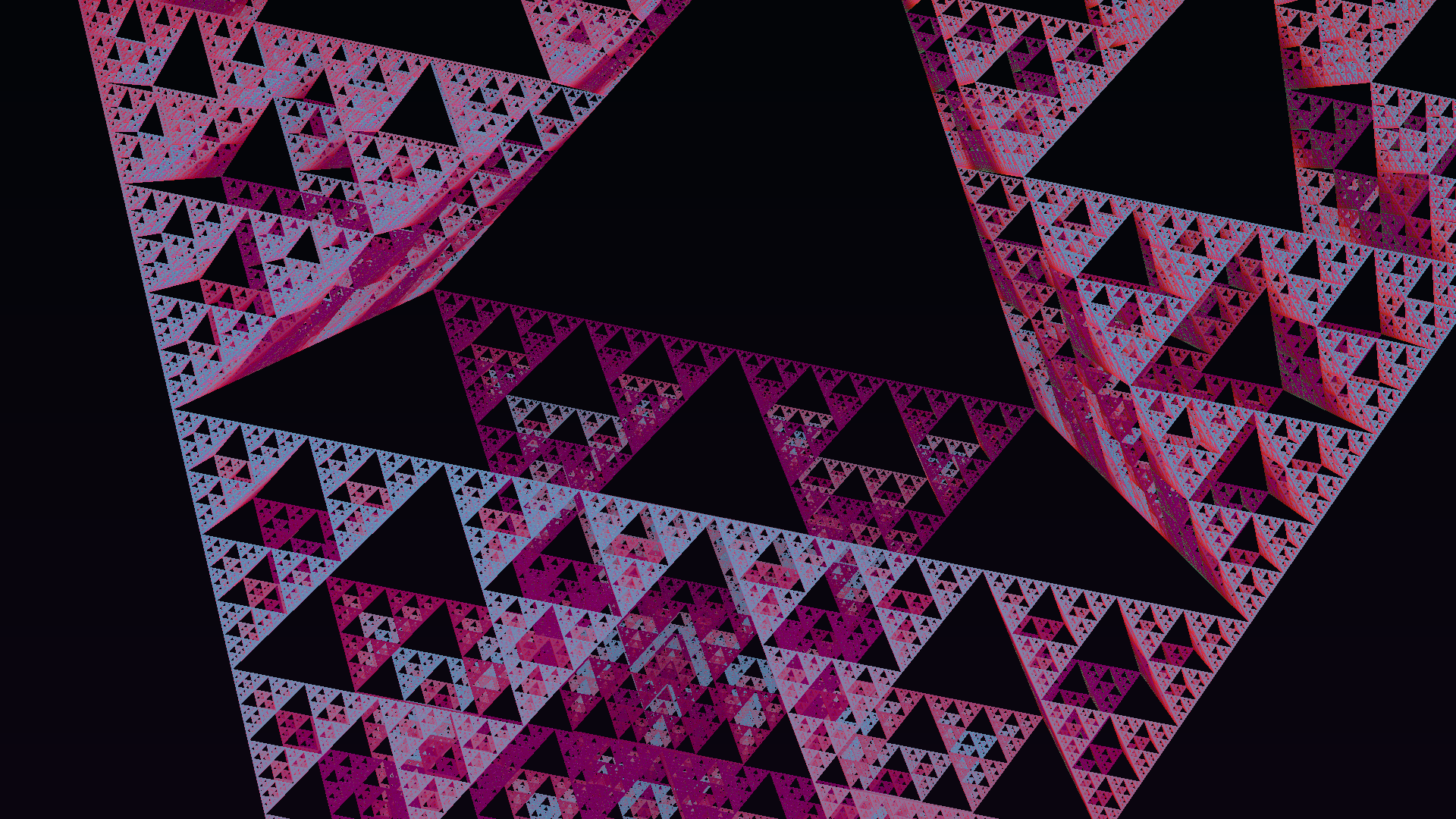
3D Sierpinski triangle (tetrahedron variant)

In 3D, the Sierpinski analogue is the tetrahedral variant. A practical DE-style implementation repeatedly folds space into a canonical tetrahedral wedge and rescales, then converts the transformed point into an approximate signed distance. ^{10 8}

Core fold step from the shader:

001inline float sierpinskiDE(float3 p, int fractalIter) {
002    float scale = 2.0;
003    float s = 1.0;
004
005    for (int i = 0; i < fractalIter; ++i) {
006        if (p.x + p.y < 0.0) p.xy = -p.yx;
007        if (p.x + p.z < 0.0) p.xz = -p.zx;
008        if (p.y + p.z < 0.0) p.yz = -p.zy;
009
010        p = p * scale - float3(1.0, 1.0, 1.0) * (scale - 1.0);
011        s *= scale;
012    }
013
014    return (length(p) - 0.6) / s;
015}

This fold logic corresponds to reflecting into symmetric half-spaces (p.x+p.y<0, etc.), then doubling scale. The s factor tracks accumulated scaling so distance remains consistent across iterations.

Raymarch integration:

001for (int i = 0; i < maxSteps; ++i) {
002    float3 p = ro + rd * t;
003    float d = sierpinskiDE(p, fractalIter);
004    if (d < hitEps) { hit = true; break; }
005    t += max(d, 0.0002) * stepScale;
006}

Shading (simplified):

001float diff = clamp(dot(n, lightDir), 0.0, 1.0);
002float rim  = pow(clamp(1.0 - dot(n, -rd), 0.0, 1.0), 2.2);
003float ao   = exp(-0.11 * t);
004col = palette(base + 0.5 * trapTone + 0.2 * diff) * ao + 0.12 * rim;

So even for this very geometric fractal, the image quality depends heavily on DE quality, hit epsilon, and normal stability.

Mandelbulb

Basic Mandelbulb

The basic Mandelbulb follows the Mandelbrot logic but in 3D spherical coordinates: convert $z$ to $(r,\theta,\phi)$, apply power $n$, convert back, and add the seed point $p$. For DE rendering, we track derivative growth dr, which yields

$$d \approx \frac{1}{2}\,\log(r)\,\frac{r}{dr}.$$

In code, the evaluator usually returns more than distance. Besides dist, we keep orbit metrics because they are useful for shading:

001struct Eval {
002    float dist;
003    float iterNorm;
004    float trap;
005    float trapAxis;
006    float drNorm;
007};

Minimal DE evaluator shape (basic bulb, no fancy variations):

001inline Eval evalBasicBulb(float3 p, float power, int maxIter) {
002    float3 z = p;
003    float dr = 1.0;
004    float r = 0.0;
005    float trap = 1e9;
006    int i = 0;
007
008    for (; i < maxIter; ++i) {
009        r = length(z);
010        trap = min(trap, r);
011        if (r > 2.0) break;
012
013        float safeR = max(r, 1e-6);
014        float theta = acos(clamp(z.z / safeR, -1.0, 1.0));
015        float phi = atan2(z.y, z.x);
016
017        dr = power * pow(safeR, power - 1.0) * dr + 1.0;
018        float zr = pow(safeR, power);
019
020        theta *= power;
021        phi   *= power;
022
023        z = zr * float3(sin(theta) * cos(phi),
024                        sin(theta) * sin(phi),
025                        cos(theta)) + p;
026    }
027
028    Eval out;
029    out.dist = 0.5 * log(max(r, 1e-6)) * r / max(dr, 1e-6);
030    out.iterNorm = float(i) / float(maxIter);
031    out.trap = trap;
032    out.trapAxis = 0.0;
033    out.drNorm = clamp(log2(max(dr, 1.0)) / 14.0, 0.0, 1.0);
034    return out;
035}

Canonical power-map step:

001float safeR = max(r, 1e-6);
002float theta = acos(clamp(z.z / safeR, -1.0, 1.0));
003float phi = atan2(z.y, z.x);
004
005dr = power * pow(safeR, power - 1.0) * dr + 1.0;
006float zr = pow(safeR, power);
007
008theta *= power;
009phi   *= power;
010
011z = zr * float3(sin(theta) * cos(phi),
012                sin(theta) * sin(phi),
013                cos(theta)) + p;

return DE:

001return 0.5 * log(max(r, 1e-6)) * r / max(dr, 1e-6);

Compared to escape-time coloring, this DE route is what makes high quality 3D shading and camera motion possible. ¹¹¹²

Raymarch usage in the basic case:

001float t = 0.0;
002for (int i = 0; i < maxSteps; ++i) {
003    float3 p = ro + rd * t;
004    Eval ev = evalBasicBulb(p, power, maxIter);
005    if (ev.dist < hitEps) { hit = true; hitEval = ev; break; }
006    t += max(ev.dist, 0.0002);
007    if (t > maxDist) break;
008}

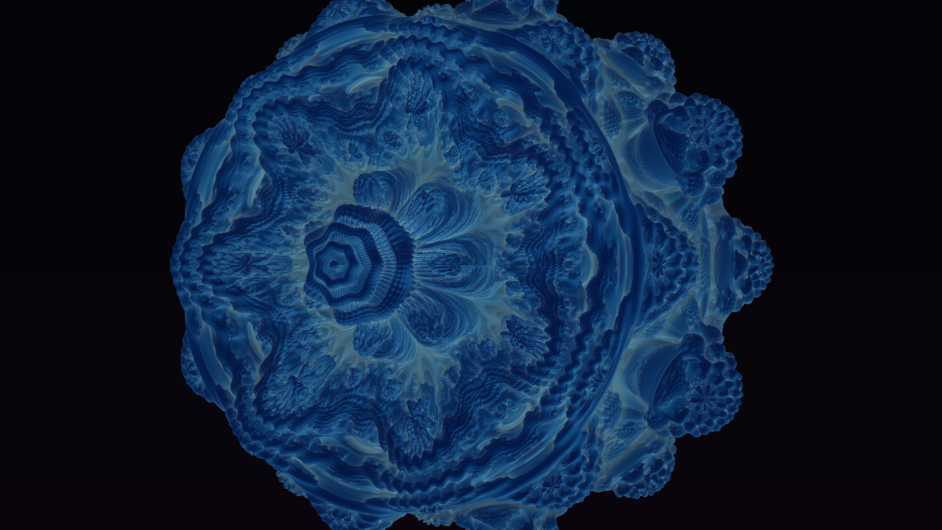
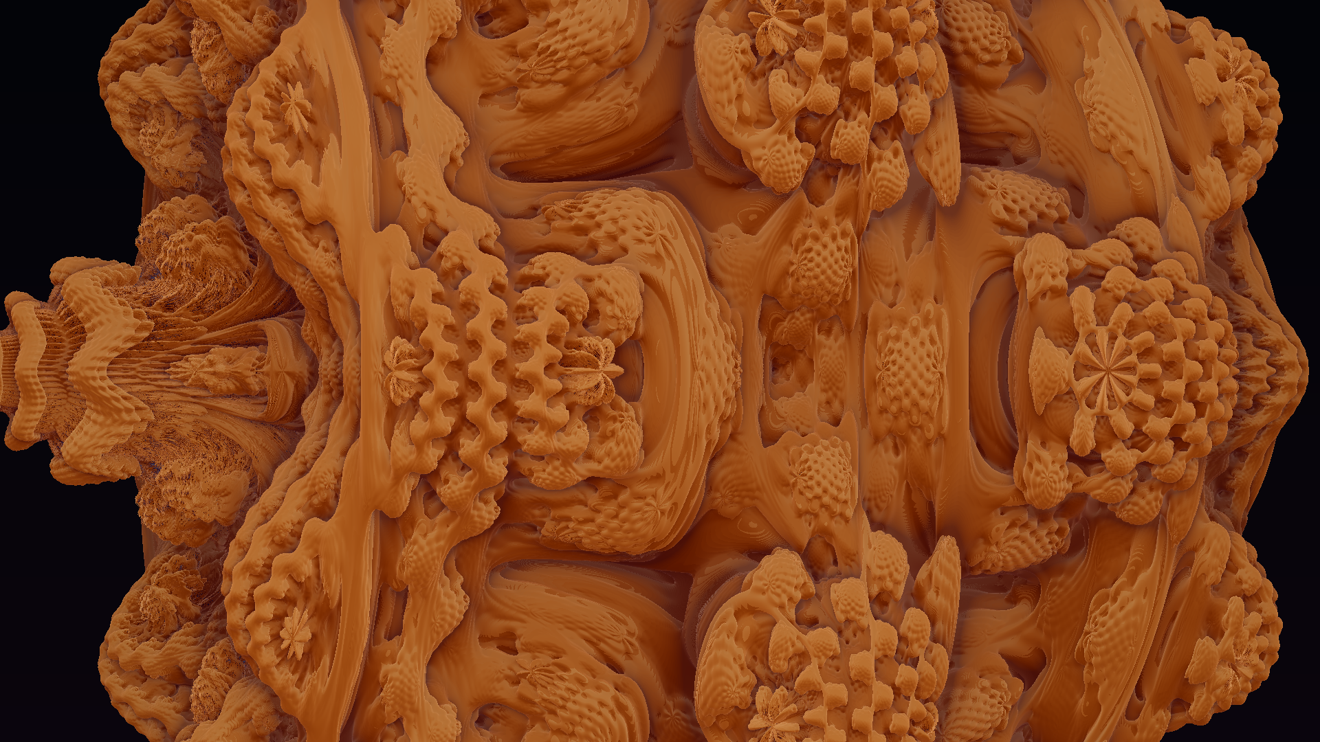
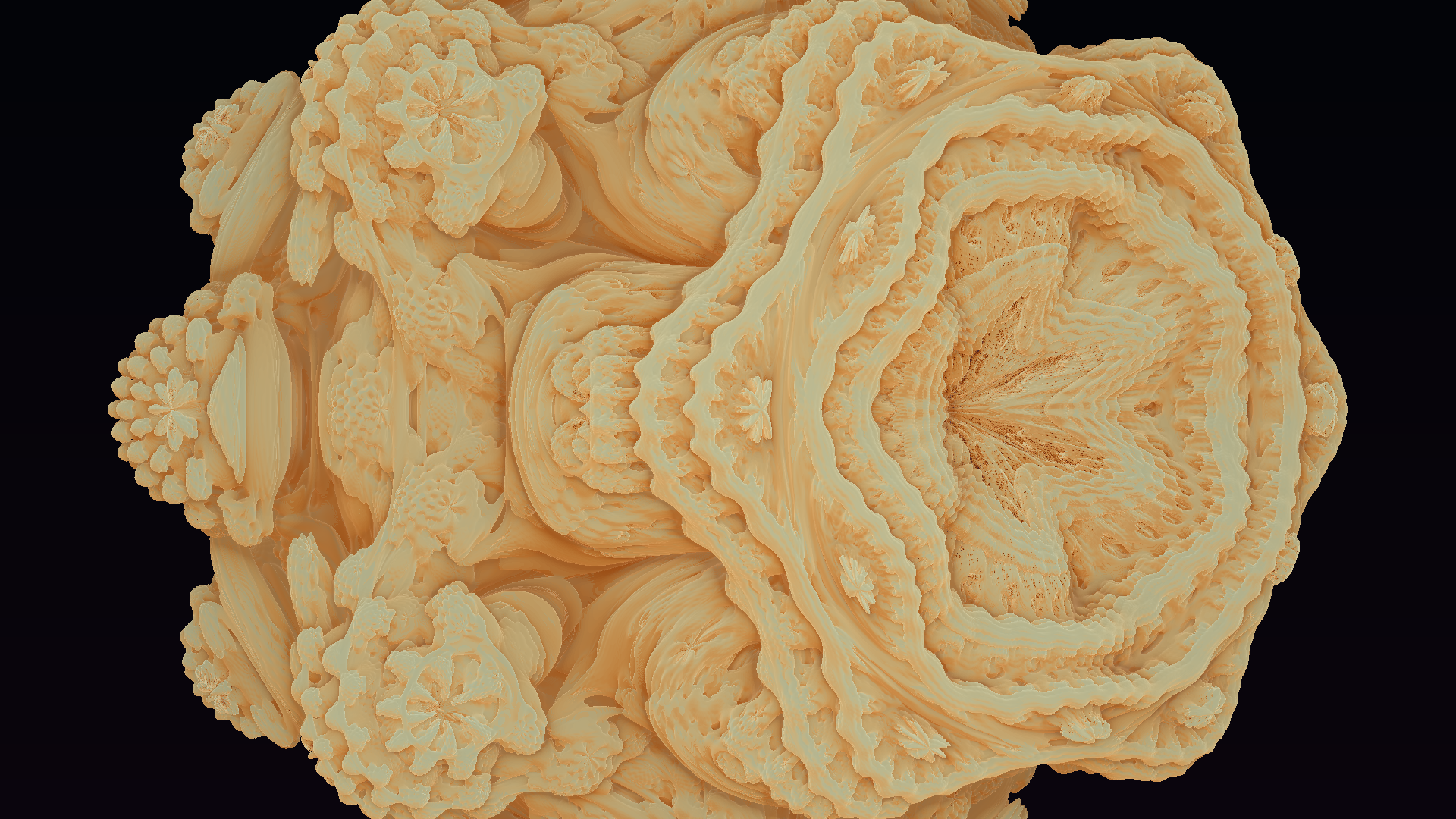
in the following, color follows orbit structure (trap, iterNorm, drNorm) and therefore stays coupled to the fractal itself. ^{8 12}

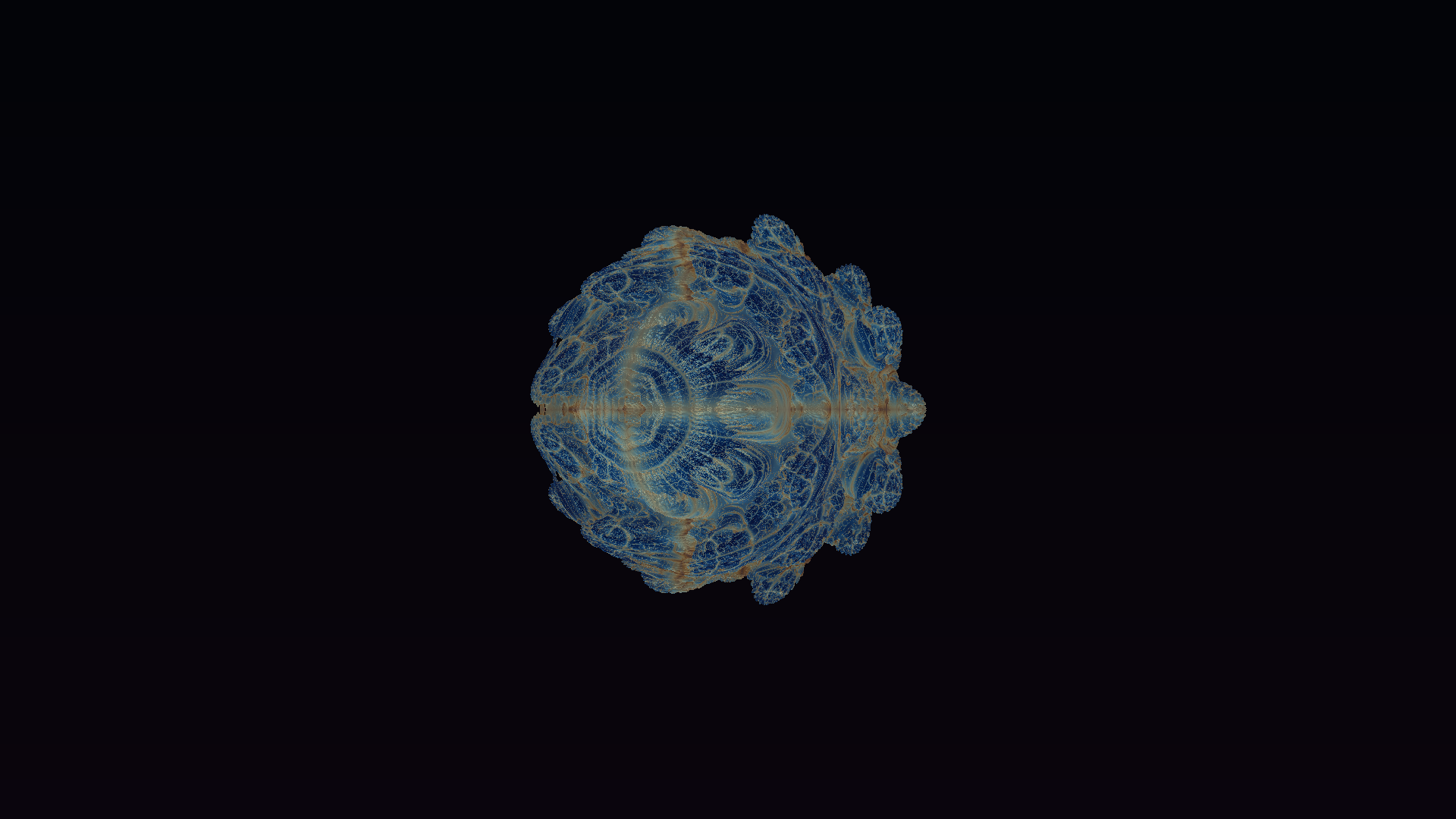
Abs-hybrid preset example:

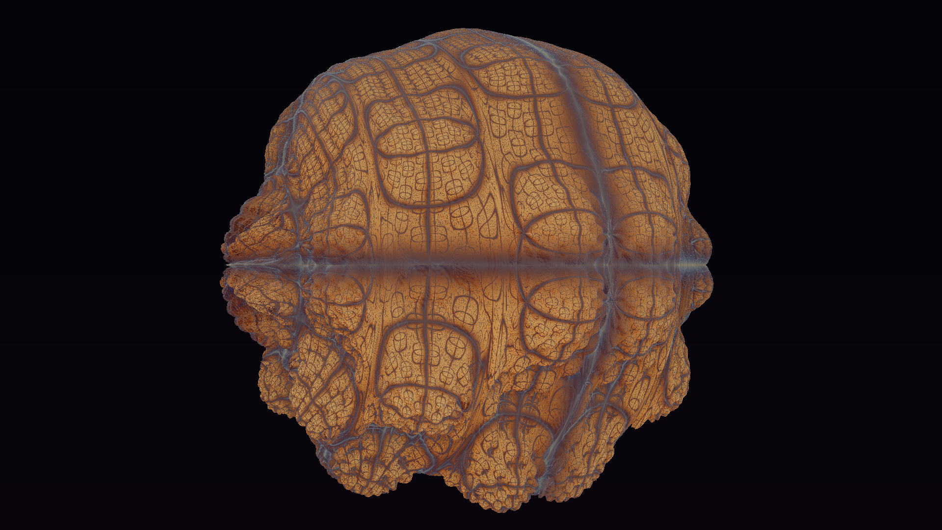
Bonus

Quaternions

Quaternions extend complex numbers from 2 to 4 components,

$$q = r + ai + bj + ck,$$

with non-commutative multiplication rules; they form a ring. For fractals, this gives a direct way to define 4D escape-time maps analogous to complex Julia sets. ¹³

4D quaternion Julia set (Bourke)

An alternative approach to higher-dimensional Julia/Mandelbrot-style sets was published by Paul Bourke: iterate

$$q_{n+1}=q_n^2+c,$$

use an escape radius around 4, and reduce dimension by slicing $\mathbb{R}^4$ with a 3D hyperplane before rendering. ¹⁴

Let

$$F_c(q)=q^2+c, \qquad q\in\mathbb{H}\cong\mathbb{R}^4,$$

with quaternion multiplication. Define the bounded-orbit set

$$K_c = \left\{q_0\in\mathbb{R}^4 : \{F_c^{\,n}(q_0)\}_{n\ge 0}\text{ is bounded}\right\},$$

and its boundary (the 4D Julia analogue) $J_c=\partial K_c$.

A direct visualization of $J_c\subset\mathbb{R}^4$ is not possible on a 2D screen, so a 3D hyperplane slice is used:

$$H_{w_0}=\{(x,y,z,w)\in\mathbb{R}^4 : w=w_0\}.$$

The visible 3D object is then

$$S_{w_0}=J_c\cap H_{w_0}.$$

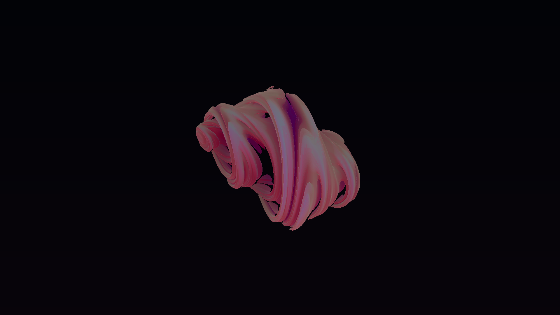
After that, standard 3D rendering applies: cast rays in $\mathbb{R}^3$ into $S_{w_0}$ and shade intersections.

The shader mirrors this math in four stages:

1. Build a 4D point from a 3D sample point and fixed slice coordinate $w_0$.
2. Iterate quaternion dynamics $q\leftarrow q^2+c$ with an escape test.
3. Convert orbit behavior into a DE-like distance estimate.
4. Raymarch in 3D using that distance field.

Minimal embedding step (3D sample point to 4D state):

001float4 q = float4(p.x, p.y, p.z, wSlice);

Minimal quaternion square snippet used in shader code:

001inline float4 qmul(float4 a, float4 b) {
002    return float4(
003        a.x*b.x - a.y*b.y - a.z*b.z - a.w*b.w,
004        a.x*b.y + a.y*b.x + a.z*b.w - a.w*b.z,
005        a.x*b.z + a.z*b.x + a.w*b.y - a.y*b.w,
006        a.x*b.w + a.w*b.x + a.y*b.z - a.z*b.y
007    );
008}
009
010q = qmul(q, q) + cParam;

Orbit loop with escape criterion (Bourke-style radius):

001float dr = 1.0;
002float r = 0.0;
003for (int i = 0; i < maxIter; ++i) {
004    r = length(q);
005    if (r > 4.0) break;
006    dr = 2.0 * r * dr + 1.0;
007    q = qmul(q, q) + cParam;
008}
009float dist = 0.5 * log(max(r, 1e-6)) * r / max(dr, 1e-6);

This dist term is then consumed by the regular 3D sphere-tracing loop.

Render:

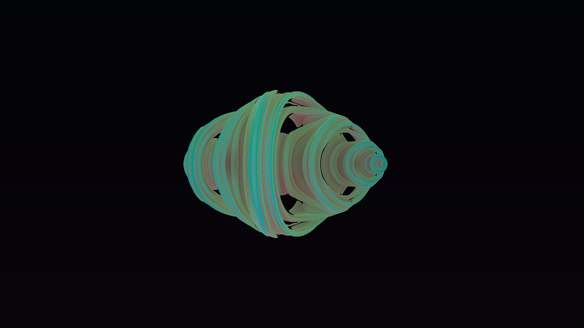
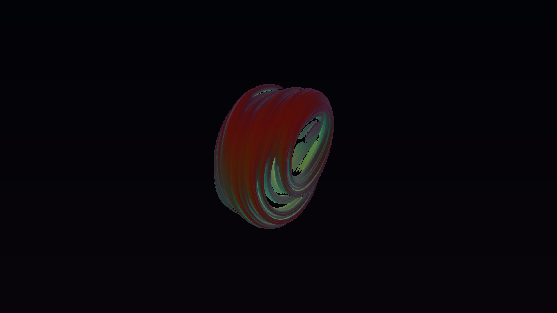
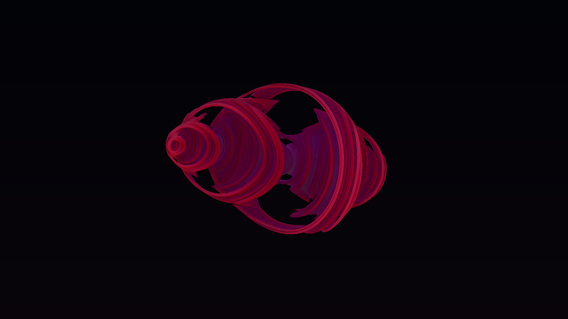
Additional quaternion Julia slices (different constants / slice parameters):

Technical Setup (Swift + Metal on macOS)

We render everything headless on macOS using swiftc + Metal ^{15 16 17} compute shaders.

1. Load/compile .metal shader source at runtime.
2. Build a compute pipeline (MTLComputePipelineState).
3. Allocate an output MTLTexture.
4. Dispatch a 2D grid (width x height) with one thread per pixel.
5. Read back texture bytes and write PNG.

Swift pipeline setup (core idea):

001let source = try String(contentsOfFile: sourcePath, encoding: .utf8)
002let library = try device.makeLibrary(source: source, options: nil)
003let fn = library.makeFunction(name: kernelName)!
004let state = try device.makeComputePipelineState(function: fn)

Uniforms are passed as a small struct:

001struct Uniforms {
002    var viewportSize: SIMD2<Float>
003    var time: Float
004    var pad0: Float
005    var p0: SIMD4<Float>
006    var p1: SIMD4<Float>
007    var p2: SIMD4<Float>
008}
009computerEncoder.setBytes(&uniforms,
010                         length: MemoryLayout<Uniforms>.stride,
011                         index: 0)

Thread dispatch:

001let w = state.threadExecutionWidth
002let h = max(1, state.maxTotalThreadsPerThreadgroup / w)
003let tpg = MTLSizeMake(w, h, 1)
004let grid = MTLSizeMake(width, height, 1)
005computerEncoder.dispatchThreads(grid, threadsPerThreadgroup: tpg)

The important implementation detail on macOS is readback: if the texture is in managed storage, a blit synchronization is required before CPU reads.¹⁸

More References

For practical fractal rendering applications and deeper implementation writeups:

• Introduction to Raymarching: ⁹
• Distance-estimated 3D fractal series: ¹⁹
• Mandelbulber overview and usage: ²⁰
• 4D quaternion Julia ray-tracer project notes: ²¹
• General path-tracer: ²²

Footnotes

1. Mandelbrot set overview: Link ↩ ↩²

2. Fractal dimension (Hausdorff and related): Link ↩

3. Barnsley fern / IFS context: Link ↩

4. Iterated Function System overview: Link ↩

5. Complex dynamics overview: Link ↩

6. Paul Bourke, SinJulia fractals: Link ↩

7. Sphere tracing overview (with original reference links): Link ↩

8. Inigo Quilez, Distance Functions and Raymarching notes: Link ↩ ↩² ↩³

9. Detailed raymarching explanation (distance fields): Link ↩ ↩²

10. Sierpinski tetrahedron context: Link ↩

11. Mandelbulb historical notes and power map: Link ↩

12. Practical DE discussion: Link ↩ ↩²

13. W. R. Hamilton, original quaternion work context: Link ↩

14. Paul Bourke, Quaternion Julia Fractals: Link ↩

15. Apple Developer Documentation, Metal: Link ↩

16. Apple Developer Documentation, MetalKit: Link ↩

17. Metal Shading Language Specification: Link ↩

18. Resource storage modes and synchronization: Link ↩

19. Distance Estimated 3D Fractals Part I: Link ↩

20. Applications for rendering fractals (Mandelbulber): Link ↩

21. 4D Quaternion Julia Set Ray Tracer (Mac/Windows): Link ↩

22. General Pathtracer: Link ↩