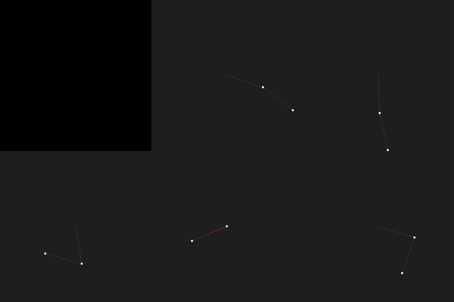
Animating a double pendulum

Simulating a double pendulum involves solving its equations of motion, which are derived from Lagrangian mechanics. These equations form a system of nonlinear second-order ordinary differential equations (ODEs).

Differential equations

The double pendulum system consists of two point masses $m_1$​ and $m_2$​, attached by rigid massless rods of lengths $l_1$​ and $l_2$​, swinging under gravity. Let $\theta_1$​ and $\theta_2$​ be the angles each pendulum makes, measured from the vertical.

$$\begin{aligned} \ddot{\theta}_1 &= \frac{ -g (2m_1 + m_2) \sin\theta_1 - m_2 g \sin(\theta_1 - 2\theta_2) - 2 \sin(\theta_1 - \theta_2) m_2 \left( \dot{\theta}_2^2 l_2 + \dot{\theta}_1^2 l_1 \cos(\theta_1 - \theta_2) \right) }{ l_1 \left( 2m_1 + m_2 - m_2 \cos(2\theta_1 - 2\theta_2) \right) } \\[1em] \ddot{\theta}_2 &= \frac{ 2 \sin(\theta_1 - \theta_2) \left( \dot{\theta}_1^2 l_1 (m_1 + m_2) + g (m_1 + m_2) \cos\theta_1 + \dot{\theta}_2^2 l_2 m_2 \cos(\theta_1 - \theta_2) \right) }{ l_2 \left( 2m_1 + m_2 - m_2 \cos(2\theta_1 - 2\theta_2) \right) } \end{aligned}$$

Since analytical solutions aren't known, we use numerical methods to approximate the pendulum's motion.

Numerical Integration of ODEs

To simulate physical systems we compute the system's state at each step using estimates of its derivatives.

Runge-Kutta

The Runge-Kutta methods are a family of iterative techniques for integrating ODEs. Commonly used is the 4th-order Runge-Kutta (RK4) method. RK4 improves upon simpler methods like Euler's by sampling the derivative multiple times at each step.

Implementation in C++

Here are the differential equations, expressed in c++:

001typedef std::vector<double> State;  
002  
003// ########### Derivatives function for RK4 ###########  
004State derivatives(const State& y) {  
005    const double theta1 = y[0];  
006    const double theta2 = y[1];  
007    const double omega1 = y[2];  
008    const double omega2 = y[3];  
009  
010    const double delta = theta2 - theta1;  
011  
012    const double den1 = (m1 + m2) * l1 - m2 * l1 * std::cos(delta) * std::cos(delta);  
013    const double den2 = (l2 / l1) * den1;  
014  
015    double domega1 = (  
016        m2 * l1 * omega1 * omega1 * std::sin(delta) * std::cos(delta) +  
017        m2 * g * std::sin(theta2) * std::cos(delta) +  
018        m2 * l2 * omega2 * omega2 * std::sin(delta) -  
019        (m1 + m2) * g * std::sin(theta1)  
020    ) / den1;  
021  
022    double domega2 = (  
023        -m2 * l2 * omega2 * omega2 * std::sin(delta) * std::cos(delta) +  
024        (m1 + m2) * (  
025            g * std::sin(theta1) * std::cos(delta) -  
026            l1 * omega1 * omega1 * std::sin(delta) -  
027            g * std::sin(theta2)  
028        )  
029    ) / den2;  
030  
031    return { omega1, omega2, domega1, domega2 };  
032}

In the full implementation, we perform one step per frame.

001// ########### RK4 integrator step ###########  
002State rk4_step(const State& y, double dt) {  
003    const State k1 = derivatives(y);  
004    State y_temp(4);  
005  
006    for (int i = 0; i < 4; ++i) y_temp[i] = y[i] + 0.5 * dt * k1[i];  
007    const State k2 = derivatives(y_temp);  
008  
009    for (int i = 0; i < 4; ++i) y_temp[i] = y[i] + 0.5 * dt * k2[i];  
010    const State k3 = derivatives(y_temp);  
011  
012    for (int i = 0; i < 4; ++i) y_temp[i] = y[i] + dt * k3[i];  
013    const State k4 = derivatives(y_temp);  
014  
015    State y_next(4);  
016    for (int i = 0; i < 4; ++i)  
017        y_next[i] = y[i] + dt / 6.0 * (k1[i] + 2 * k2[i] + 2 * k3[i] + k4[i]);  
018  
019    return y_next;  
020}

Result